
Boundary conditions in finite element analysis
Discussion of different possible boundary conditions and their significance
The boundary conditions are investigated on a single pole of a surface-mounted permanent magnet motor with inner rotor under no-load conditions It is a 10 kW motor designed for the traction of an electric forklift. Its rated torque is 60 Nm and rated speed 1500 rpm. The motor should run up to 3750 rpm in constant power by weakening the flux. The power is supplied by a 48 V battery. It has 4 poles and 3 slots/pole/phase. The current density is low with 4 A/mm2 since the motor is not cooled with any fans.
What happens if we don't apply any boundary conditions?
Fig. 1 shows what happens if we don't apply any boundary conditions. As you can see, all flux lines are perpendicular to the boundaries where they cross them (90 degrees). This natural boundary condition is often referred to as Neumann boundary condition. However, in our case it is not really what we are looking for, since we know that the flux lines should mostly stay within the active part of the electrical machine and not cross the inner and outer boundaries.
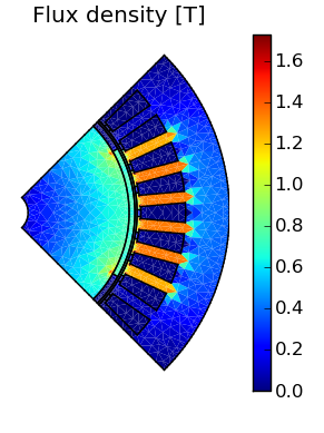 | 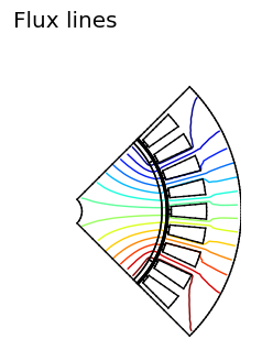 |
| Fig. 1 Flux density and flux lines with Neumann boundary conditions on all sides. | |
How can we prevent that the flux lines cross the boundary?
Flux lines are equipotential lines of the magnetic vector potential. So in order to prevent the flux lines from crossing the boundaries, we fix the magnetic vector potential to zero along the boundaries. This boundary condition is often referred to as homogeneous Dirichlet condition. As you can see in Fig. 2, our strategy was a full success and no flux is crossing the inner or outer barriers any more. However, the flux lines are still not looking correct and we should further investigate the possibilities for the upper and lower boundaries.
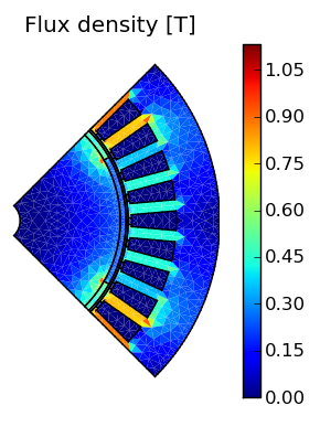 | 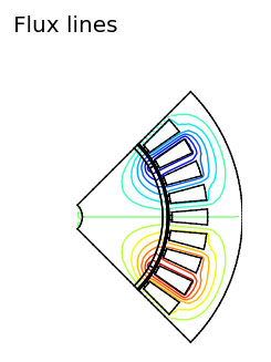 |
| Fig. 2 Flux density and flux lines with Dirichlet boundary conditions on all sides. | |
What about periodic boundary conditions?
Was not one of the reasons that we were investigating boundary conditions, that we were cutting the electrical machine cross section in parts and only analysing a single part of it due to machine symmetries? That means that the flux should be repeated in the machine. Consequently, we should be able to use periodic boundary conditions, where the magnetic vector potential in every point on the lower boundary is the same as the magnetic vector potential on the corresponding point on the upper boundary. Fig. 3 shows how the flux density and flux lines look like for such an even periodic boundary condition.
| | |
| Fig. 3 Flux density and flux lines with EVEN periodic boundary conditions on the upper and lower boundaries. | |
Ooops, that did not change anything. Even periodic boundary conditions work fine for an even number of poles simulated. For an odd number of poles, however, one should use odd periodic boundary conditions. In such a way, the magnetic vector potential in every point on the lower boundary is the negative value of the magnetic vector potential on the corresponding point on the upper boundary. As shown in Fig. 4, flux densities and flux lines look just perfect now (Please notice that in this specific case, the same result could be achieved with Neumann instead of odd periodic boundary conditions, assuming Dirichlet conditions on the inner and outer boundaries).
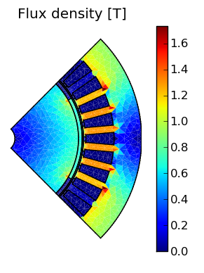 | 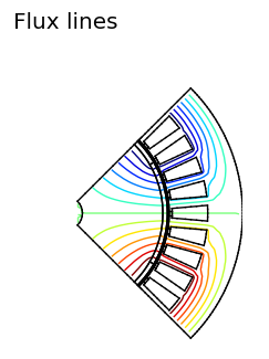 |
| Fig. 4 Flux density and flux lines with ODD periodic boundary conditions on the upper and lower boundaries. | |
Conclusions
Boundary conditions in finite element analysis of electrical machines are generally quite straight-forward. When generating the mesh, it is asvisable to generate the mesh for half a stator slot and half a rotor pole only. Afterwards it should be mirrored, copied and reassembled with a suitable airgap mesh. This has the advantage that the mesh is very homogeneous and some systematic errors due to the finite element method can be avoided. In addition, the finite element domain can often be reduced due to symmetries in the electrical machine and boundary conditions can be easily applied.
Read about another glossary term